Space Ornithology
A Webpage by Roger L. Mansfield ("Astroger")
Introduction. Back in 1987 I wrote a computer program to predict the naked-eye visibility of near-Earth satellites. Twenty years before that, when I started my space career as a weather satellite orbital analyst, we called our on-orbit satellites "birds." So I decided to call the program SPACE BIRDS.
Sky Publishing Corporation, publisher of
Sky & Telescope magazine, marketed
SPACE BIRDS to the readership during the period 1988-1991. During
that same four-year period, I published a
quarterly Space Ornithology Newsletter to support SPACE BIRDS
program purchasers.
This webpage provides:
(a) links to the first four quarterly Space Ornithology newsletters and the first three pages of
the SPACE BIRDS user's manual,
(b) an index to all sixteen newsletters, and finally,
(c) it tells how you can obtain a Space Ornithology Kit consisting of a CD-ROM containing
the SPACE BIRDS computer program, all sixteen quarterly newsletters, and a copy of my paper, "Naked-Eye
Acquisition of Visible Near-Earth Satellites" (AAS Paper 87-449, Kalispell, Montana, August 10, 1987),
plus a printed copy of the SPACE BIRDS User's Manual.
Space Ornithology Newsletters for 1988. Click on
SON1988.pdf
to open a PDF slideshow of the first four quarterly Space Ornithology newsletters.
But before you do, please note:
1. When the Adobe Acrobat Reader asks you if you want it to go to full screen mode, click
"Yes." You can hit the escape key at any time to go back to the Acrobat Reader frame.
2. Use the keyboard's right arrow and left arrow keys to page forward and back,
respectively, through the slide show. The space bar acts like the right arrow key.
Space Ornithology Defined. If you are not already familiar with the SPACE BIRDS computer
program, you might be wondering, "what is space ornithology?" I answered this question, somewhat
tongue-in-cheek*, by coining the term and defining it in the first two pages of the SPACE BIRDS User's
Manual. Click on
Primer.pdf
to see the cover page and the two "A Primer on Space Ornithology" pages.
*Did you notice the month and day, in the date given on the last line of the primer? -- There is no
such society as the "Maculate Order of Space Ornithologists" (M.O.S.O.)
The Space Ornithology Newsletter (SON) was published quarterly on the 15th of January, April, July, and
October during the years 1988 through 1991, as information for SPACE BIRDS computer program purchasers.
Each newsletter typically contained a feature article followed by "Tips for Birdbaggers" and "The Space
Ornithologist's Library."
January 1988 - International Space Year (ISY). This brief issue (1 page) told of prospects for
ISY 1992 as they looked in early 1988, when the SPACE BIRDS computer program was first introduced.
April 1988 - Space Ornithology: A New Direction for Skywatchers. This longest issue of all (8
pp.) offset the brevity of the inaugural issue by defining "space bird" and "space ornithology," by
surveying the "space bird population," and by setting precedents for the arrangement of subject matter
in subsequent newsletters.
July 1988 - Orbital Elements: the Mathematical Description of a Space Bird's Flight. Treated
orbital elements in general and NASA 2-line orbital elements in particular. Included information about
the Mir Watch program for observing the second Soviet space station.
October 1988 - Locating Space Birds: Ground Traces and Look Angles. Provided information about
how satellites are located on Earth's surface and in the sky, as a supplement to the SPACE BIRDS
manual. ("Dear Space Enthusiast" letter, dated October 15, 1988, is appended to this last SON for
1988.)
January 1989 - A Tutorial on Running the Space Birds Program. Showed and discussed sample Run
Control Information file setups for weather satellites. Treated "daylight visibility" and other special
options and settings not documented in the SPACE BIRDS manual.
April 1989 - Letters from and Air & Space Ornithologist. Provided responses to SPACE BIRDS
questions from an avid birder and newly experienced "space birder" who also happened to be a professor
of psychology at Tulane University in New Orleans.
July 1989 - Sky Trace Plotting Charts I: North and South Polar Equidistant Projections.
Described charts especially drawn for the plotting of sky traces. Provided 8.5"x11" northern and
southern hemisphere charts on acid-free-stock.
October 1989 - Sky Trace Plotting Charts II: The Rectangular Projection. Described a novel
rectangular chart drawn especially for the plotting of sky traces. Provided 11"x17" unbiased
rectangular chart on acid-free stock.
January 1990 - Remote Sensing from Earth-Orbital Space Platforms. This newsletter called
attention to the many active or planned satellites which turn their video cameras toward Earth or
space, either to tell us more about our earthly environment, or to solve the mysteries of distant
space. Included information about NASA's Great Observatories.
April 1990 - An HP7475A Plotter Utility for Drawing Sky Traces. Told how to use a
Hewlett-Packard plotter, or your own dot-matrix printer/plotter emulator software, to prepare
publication-quality charts of the paths of space birds against the background of the stars.
July 1990 - The Hubble Space Telescope. Told about the history, purpose, characteristics, ground
support, and science institute for what was to become one of the world's most foremost scientific
instruments. (Despite the figure error in the primary mirror, which was eventually corrected, this
wondrous instrument achieved its full potential in the subsequent decade.)
October 1990 - The Soviet Space Stations. This newsletter described the Salyut 7 and Mir space
stations; the Soyuz transport vehicles; the Progress resupply missions; Kvant 1 and 2; Kristall; the
brave cosmonauts who have carried out successful and sustained Soviet manned activities at 51.6 degrees
orbital inclination since 1971.
January 1991 - Space Surveillance: Maintaining the Space Catalog. Based upon author's 15 years
of practical experience in developing the mathematics and computer programs used to keep track of
everything in Earth orbit, this issue describes the mathematical building blocks of space surveillance.
(Cover letter topic: tracking the first Galileo close-Earth flyby.)
April 1991 - The Gamma-Ray Observatory. About NASA's second "Great Observatory," which was
successfully deployed from the Space Shuttle Atlantis on April 8, 1991. (Cover letter topics: decay of
Salyut 7's orbit; NASA's High Interest, Weather, and Amateur satellite groups.)
July 1991 - Observing Geostationary Satellites. This issue dealt with finding and photographing
"geosats;" showed how to forecast a geosat's fixed directions relative to a given earthbound observer
using the geosat's longitude. (Cover letter topic: Space Ornithology Newsletters to be discontinued
after issue of October 15, 1991. Gave reasons why.)
October 1991 - The Roentgensatellit (X-Ray Satellite). More about the German-British-U.S. space
mission now beginning to report back to the international scientific community. Also news of NASA's new
Remote Bulletin Board Service for orbital elements; ISY 1992 and Galileo's Second Close-Earth Flyby;
GOES Woes; Mission to Planet Earth Update; Gamma-Ray Observatory Update. (Cover letter topic: this
index to all space ornithology newsletters issued 1988-1991.)
The Space Ornithology Kit consists of a CD-ROM and printed materials. The WinZip executable on the CD will write about 8 Megabytes of content to your computer's hard disk. Suggestion: unzip to a flash drive for maximum portability and ease of use.
Provided on CD-ROM:
1. SPACE BIRDS Computer Program, Version 12.
Warning: This program is not "user friendly"
by today's standards. It was designed back
in the days of MS-DOS. That is, it was designed
to run on the MS-DOS command line of an
IBM PC, using a text editor to prepare input
files and view output files.
SPACE BIRDS can be run as a DOS program at
the DOS prompt, or executed directly from its icon
in its Windows folder.
SPACE BIRDS runs under all DOS versions and has
been verified to run under Windows 98SE, 2000, XP,
and Vista.
During 1988-1991, SPACE BIRDS was shipped with
the PC-Write text editor, for use in preparing
input files and viewing output files. Windows
users can now better use the Windows accessory
programs Notepad and Wordpad for this same
purpose.
2. SPACE Ornithology Newsletters 1988-1991.
One PDF "slide show" document per year
(four quarterly issues per year).
3. A copy of my AAS 87-449 paper, "Naked-Eye
Acquisition of Visible Near-Earth Satellites,"
dated August 10, 1987 (with corrections dated
March 10, 1998).
Provided as printed materials:
4. Quick Guide to Running SPACE BIRDS under
Windows.
5. SPACE BIRDS Manual, 43 pages.
Postal mailing address:
P.O. Box 885
Palmer Lake, CO 80133-0885
U.S.A.
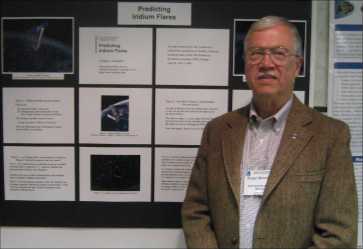
"Predicting Iridium Flares" Presentation at DDA Conference, Boulder, Colorado, April 30, 2008 -- See
http://astroger.com/
Case Study 1: Iridium Birds and Flares. The Iridium constellation of 66 operational global mobile
telephony satellites is arguably the most exciting "flock" of space birds that space ornithologists can
study right now. This is because each Iridium satellite has two highly reflective solar panels, plus
three large Main Mission Antennas (MMAs) that can reflect sunlight back to earthbound observers in a
way that can be predicted. Also, the spacecraft body itself, which is triangular in cross-section,
reflects sunlight well.
In the past two years I have put several pieces of content online as regards Iridium satellite
observing, to include an illustration of a typical Iridium satellite and some of the mathematical
details of flare prediction. Also, Tom Bisque (of
Software Bisque, Inc.)
has captured some really amazing videos of Iridium flares using his Wright-Schmidt telescope and
Paramount ME robotic telescope mount -- see the related links and references at the end of this
case study.
What I want to do now is to:
(a) tell you how to predict Iridium flares using Software Bisque's new
TheSkyX
computer program, and then
(b) show you how the SPACE BIRDS program provides a concise summary of just about everything a
seasoned satellite orbital analyst might want to know as regards Iridium satellite visibility --
especially before observing a visible pass during which an Iridium bird is predicted to flare. (And of
course, the Iridium birds are just one class of space bird that you can study with SPACE BIRDS.)
I'm going to resort now to the format that every experienced space operations analyst uses when working
a satellite pass: an operational checklist.
__1. Go to T.S. Kelso's Celestrak website, at
http://celestrak.com,
and download the three-line orbital elements (TLE) for the Iridium satellites.
By "download" I mean: when your browser is displaying the Iridium birds' orbital elements in the window
presented by Celestrak, (a) "select all" and "copy" the elements to the Windows clipboard, (b) then
open a Windows Notepad window, "paste" the elements there, and (c) "save" the elements to a Notepad
text file.
When I took this step on October 1, 2008, I named my own Notepad file "IRIDIUM CELESTRAK
2008-10-01.txt".
__2. Launch TheSkyX and predict the Iridium flares visible from your observing location
over the next seven days.
To do this, you need to go to TheSkyX's Input menu to set the location and date (in this case, October
1, 2008), and then click on the Satellites submenu to import the TLE from the file you saved in
Checklist Step 1.
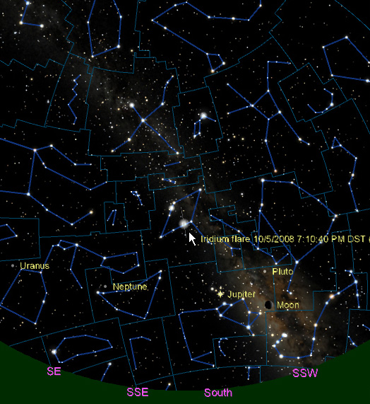
When you have imported the Iridium TLE, click on the Iridium Satellites tab and then click on Find
Flares. When I did so, I found a magnitude -2.9 flare was predicted on Sunday, October 5, 2008. Then I
clicked on the Watch Flare button to see an animation of the flare. Below is a screen capture that I
obtained from TheSkyX's Watch Flare animation.
Figure. Iridium 65 flare visible from Colorado Springs, Colorado U.S.A. on October 5, 2008,
as predicted and depicted by Software Bisque's TheSkyX.
__3. Create Orbital Elements, Observer Location, and Run Control
Information files for SPACE BIRDS, for a day on which an Iridium bird of interest will flare.
To create the Orbital Elements file, I opened the Notepad TLE file from Checklist Step 1, searched for
the Iridium 65 TLE, then copied/pasted the TLE to a text file that I named IRIDSAT.TXT. Here, in
boldface type, is the text of that file:
I had already prepared the Observer Location file -- its name is COS.TXT. Here, in boldface
type, is the text of that file:
I named the Run Control Information file RUN.TXT, and it looks like this:
Note that the start day is counted from the beginning of the year, i.e., January 1 is day 1, and
October 1, 2008 is day 279, since 2008 is a leap year. (A table of days since the beginning of the year
is given on p. 20 of the SPACE BIRDS user's manual.)
__4. Run SPACE BIRDS, specifying the three files IRIDSAT.TXT, COS.TXT, RUN.TXT.
Output went to the SPACE BIRDS output file AVES.OUT, and it looks like this:
Please note the following:
a. I adjusted the run control information so that the visible points would be output every 20 seconds,
and in particular, at 19:10:40 MDT. Also, I set the twilight threshold to 0.0 minutes. It normally
would be about 30 minutes, but this bird rises less than 30 minutes after sunset (as you can see from
the AVES.OUT output).
b. Note that SPACE BIRDS and TheSkyX don't give exactly the same azimuth and elevation at 19:10:40 MDT.
This is because TheSkyX uses the SGP4 orbit propagation model, while SPACE BIRDS uses the much
simpler (to understand and to implement), but less accurate GP1 model. The GP1 model is
documented in my textbook,
Topics in Astrodynamics,
and in my 1987 AAS paper, as supplied with the Space Ornithology Kit.
c. SPACE BIRDS tells me that the satellite is visible, at better than 50% illumination by the sun, from
the time it rises above 10 degrees elevation, all the way up to the time it sets below 10 degrees
elevation, a total of about ten minutes of naked-eye visibility.
So if I track the satellite with the naked eye or binoculars, I should be able to see the entire pass,
and I will be treated with a flare at 7:10:40 p.m. The SPACE BIRDS summary tells me that the Iridium
satellite number is 25288, that it is on orbital revolution 54977, and that the ascending nodal
crossing time and west longitude were 18:30:03 (24-hour clock) and 88.8 degrees, respectively.
d. Iridium birds are easy to observe, and interesting to observe, even when no flare is predicted on a
given pass of interest. This is because flares are only reliably predicted for the MMAs, and possibly
even the solar panels themselves (if you have access to precise information about solar panel
orientation as a function of time), but the spacecraft body by itself can generate unpredicted flashes
of reflected sunlight.
e. Although we set up the SPACE BIRDS input files here for just one satellite, we can in fact set up
SPACE BIRDS to generate visibility data (pass data only, not flares -- you need TheSkyX for the flare
predictions) for the entire Iridium satellite constellation.
We can do this by employing SPACE BIRDS in "queue mode." In queue mode, the entire file from Checklist
Step 1 is used as the Orbital Elements input file. Suppose that there are 92 satellites (operational,
non-operational, and spare). Then we copy the two observer location lines 91 times in the Observer
Location file, and copy the run control line 91 times in the Run Control information file, followed by
one blank line to terminate the program.
In other words, queue mode means that we can "queue up" visibility prediction requests for varying
satellite, observer, and run control combinations. Admittedly, this is cumbersome by today's standards,
but SPACE BIRDS was originally designed at a time when generating a day's visibility data on 92
satellites was unthinkable -- it would have taken a prohibitive amount of machine time on a desktop
computer with the the Intel 8088/8087 chip set. Nowadays, the task takes just takes a few seconds.
Case Study Summary. Although the SPACE BIRDS program is more than two decades old now, there is
much information, concisely presented, in the SPACE BIRDS output summary to please today's orbital
analyst. And even though SPACE BIRDS is an MS-DOS program, the Windows Notepad editor makes it easy to
set up the input files and run the program from a Windows folder.
Related Links and References
1. Predicting Iridium Flares was the title of both my DDA 2008 Boulder presentation and a
subsequent article in the
May 2008 issue of PTC Express,
the monthly online newsletter for Pro/Engineer, Mathcad, and other Parametric Technology Corporation
(PTC) product users. You can download the presentation and publicity flyer directly from the following
links:
Presentation,
Publicity Flyer.
2. Tom Bisque, one of the four
Brothers Bisque
(from left to right in the photo: Matt, Tom, Dan, and Steve),
has done some truly remarkable satellite tracking with his
robotic telescope setup,
which uses TheSky for telescope control via its
Paramount ME telescope mount.
You can find out more by visiting
Tom's Corner.
3. T.S. ("TS") Kelso has produced a trilogy of webinars on satellite visibility (November 28, 2006),
Iridium flares (December 5, 2006), and satellite transits of the Sun and Moon (December 12, 2006). See
AGI Webinars.
By the way, TS provides the operational status of the Iridium birds at his Celestrak website:
[+] denotes "operational," [-] denotes "non-operational," and [S] denotes "spare."
The status is on the same line as the satellite common name, i.e., it is on the first line of the TLE.
(Did you notice the [+] on the SATELLITE NAME line of the SPACE BIRDS output summary?)
Why is operational status important to a visual observer? Because (a) operational Iridium birds flare
predictably; (b) non-operational birds are not maintained at nominal "long axis down, MMA#1 forward"
attitude, and so do not flare predictably; (c) spare Iridium birds are kept in lower orbits, but are
boosted to operational altitude before being used for the global mobile telephony mission.
Tom, TS, and I have all observed Iridium spares to flare predictably. This obviously implies that the
on-orbit attitude of each of the Iridium spares is being maintained according to the "long axis down, MMA#1
forward" control law.
Case Study 2: Angles-Only Orbit Determination. There are several widely-known, well-documented angles-only orbit determination methods out there for artificial Earth satellites: Gauss, Lagrange-Gauss-Gibbs, and Laplace readily come to mind.
But the method that I like best is not on this short list. The method that I like best is Herget's method.
Herget's Method is well-known to those who use Earth-based telescopes to measure the celestial positions of comets and asteroids (thanks to Tony Danby, and more recently, to Bill J. Gray and his Project Pluto). But it is not so well-known to those of us who determine artificial Earth satellite orbits. (Perhaps in the not-too-distant future it will be.)
Therefore, in this case study I will apply Herget's method to the problem of determining a preliminary orbit for a LEO (low-Earth orbit) satellite.
The basic idea of Herget's method is to take a set of topocentric RA (right ascension) and DEC (declination) measurements of an asteroid or comet, guess the topocentric distances rho1 and rho2, and then iterate on these initial distance estimates via equations that seek to minimize their residuals in the sense of "observed minus computed." Herget's method is thus a two-parameter fit of rho1 and rho2 to as many observations as are available.
Embedded within Herget's method is Gauss's two-position-vector-and-time (TPV&T) orbit determination method. Gauss's TPV&T method solves this problem: given two position vectors of the secondary in a two-body system, and given the time of flight of the secondary from the first position to the second, find the velocity of the secondary at its first position.
Upon analyzing the mathematics of Herget's method, starting with Herget's original article in the Astronomical Journal (AJ, 1965), I found that I could write Gauss's hypergeometric X-function as a quotient of c-functions, whereas Herget, in his AJ article, uses the older truncated-series representation of the X-function.
Further, my own adaptation of Herget's method uses f and g functions of Stumpff's c-functions to propagate position and velocity, and thus it does not assume that the orbit is elliptical. The orbit can be parabolic or hyperbolic, and this does not affect the mathematics or the solution vector. (The derivation of my improvements to Gauss's TPV&T method, which also therefore constitute improvements to Herget's method, can be found in Chapter 14 of my textbook,
Topics in Astrodynamics.)
An advantage of Herget's method over the other three methods cited above is that it can use all of the available observations in a given track. One does not have to judiciously pick out just three angles-only observations. Plus, one gets a two-parameter fit over all available observations.
To build a LEO test case that illustrates Herget's method, we need look no farther than the SPACE BIRDS output for the Iridium 65 satellite dealt with in Case Study 1. There are 31 angles-only "observations" in that case study. Since the SPACE BIRDS-predicted RA "measurements" are rounded to the nearest minute of time, and the DEC "measurements" are rounded to the nearest minute of arc, they have built into them a random error of +/- half a time-minute in RA, and a random error of +/- half an arc-minute in DEC. Observations comprised of these two measurements should not, therefore, be called perfect observations.
My implementation of Herget's method for artificial Earth satellites, called GH1/GHC, gives the following elements after three GHC iterations (final RMS error was 1.251 km). Epoch is at the time of the first observation.
*At first glance it would appear that the GH1/GHC argument of perigee and mean anomaly do not agree with those predicted by SPACE BIRDS.
However, since the eccentricity is quite small, we need to add the argument of perigee to the mean anomaly in both cases, thereby obtaining the mean argument of latitude. We see, then, that on the line labeled MEAN ARG. OF LATITUDE, we get good agreement between Herget's method and SPACE BIRDS.
**Two-line elements were propagated to the time of first observation via the GP1 model, then position and velocity at this time were transformed to classical elements.
***My implementation of Herget's method is documented on the Web at
Mathcad Worksheets by Astroger.
(To find the downloadable files, Google with quotes: "Herget's Method with Cassini's Earth Flyby" -- GH1.mcd is the geocentric Herget's method manual initiation worksheet; GHC.mcd is the manual iteration worksheet.) If you have trouble finding and downloading the two worksheets at PTC's new Mathcad website, then contact me directly by e-mail.
Conclusion. We can conclude from Case Study 2 that Herget's method, despite being only a two-parameter fit, leads to a good, single-track preliminary orbit solution for the LEO example chosen.
Case Study 3: Differential Correction of an Orbit. Herget's method, as noted in Case Study 2, does a two-parameter fit to all of the available observations. Differential correction (DC), as done for this case study, constitutes a six-parameter fit (position and velocity).
The initial estimate needed to start the DC is the Herget's method solution from the previous case study. Here are the results after two GDC iterations (final RMS error was 0.895 km).
*Two-line elements were propagated to the time of first observation via the GP1 model, then position and velocity at this time were transformed to classical elements.
**At first glance it would appear that the Herget's method argument of perigee and mean anomaly agree reasonably well with the GD1/GDC argument of perigee and mean anomaly, but not with those same elements as predicted by SPACE BIRDS.
However, since the eccentricity is quite small, we need to add the argument of perigee and mean anomaly in all three cases, thereby obtaining the mean argument of latitude, and look for agreement there. We see, then, that on the line labeled MEAN ARG. OF LATITUDE, we do get good agreement for all three sets of predictions.
***My implementation of a single-track, geocentric, two-body DC is called GD1/GDC and is documented on the Web at
Mathcad Worksheets by Astroger.
(To find the downloadable files, Google with quotes: "Tracking Data Reduction for Galileo's Earth 1 Flyby" -- GD1.mcd is the geocentric DC manual initiation worksheet; GDC.mcd is the geocentric DC manual iteration worksheet.) If you have trouble finding and downloading the two worksheets at PTC's new Mathcad website, then contact me directly by e-mail.
Conclusion. We can conclude from Case Study 3 that the Herget's method solution, as obtained from Case Study 2, can be improved somewhat via a DC that employs two-body orbital modeling.
However, we should note that in the real world, the observations would be actual observations from an optical sensor, and the DC mathematics would not be limited to two-body modeling. The DC would incorporate at least SGP or SGP4 orbital modeling, and would therefore account for orbital perturbations by atmospheric drag as well as by the J2, J3, and J4 terms of the geopotential.
(c) 2008-2018 by Astronomical Data Service. Last updated 2018 October 17.
Index to Space Ornithology Newsletters 1988-1991
Space Ornithology Kit
How to Purchase the Space Ornithology Kit
IRIDIUM 65 [+]
1 25288U 98021D   08274.64871166 -.00000065  00000-0 -30155-4 0  2797
2 25288  86.3913 113.6449 0002272  82.5170 277.6282 14.34218014549001
COLORADO SPRINGS, COLORADO U.S.A.
+38.833  -104.817   1.981  -06.00   COLOSPGS
   LATI     LONGI  HEIGHT   D UTC   ABBREV'D
   TUDE      TUDE    (KM)    (HR)   LOCATION
   F7.3     F10.3    F8.3    F8.2     3X, A8

o ONLY THE FIRST TWO LINES ARE READ BY THE PROGRAM, UNLESS IN QUEUE MODE.
o FIRST LINE IS TEXT DESCRIPTOR FOR YOUR LOCATION, UP TO 72 CHARACTERS.
o INPUT LATITUDE NEGATIVE IF SOUTH; INPUT LONGITUDE NEGATIVE IF WEST.
o D UTC IN HOURS IS  -5.00 FOR EST;   -6.00 FOR CST; -7.00 FOR MST;
                     -8.00 FOR PST;  -9.00 FOR AST; -10.00 FOR HST.
  (ADD ONE HOUR FOR DAYLIGHT SAVING TIME.)
o ABBREVIATED LOCATION DESCRIPTOR CAN CONTAIN UP TO 8 CHARACTERS.
  279-    1  3.00     YES    YES   3D3D  10.00   10.00     YES   0.00      NO

START   NBR  PNTS    WANT   WANT   PASS LOWEST  LOWEST  VISBLE    TWI  INVISB
  DAY    OF   PER  SCREEN   DISK   MODE     EL  MDP EL  POINTS THRESH    MIDP
       DAYS   MIN  OUTPUT  OUTPT   CODE  (DEG)   (DEG)    ONLY  (MIN)  REJECT
   I5    I6  F6.2   5X,A3  4X,A3  3X,A4   F7.2    F8.2   5X,A3   F7.2   5X,A3

o ONLY FIRST TWO LINES ARE READ BY PROGRAM; SECOND LINE MUST BE BLANK UNLESS
  IN QUEUE MODE. ALL DATA SHOULD BE RIGHT-ALIGNED IN FIELDS.
o PASS MODE CODE: _ALL=ALL PASSES;       _DAY=ALL DAY PASSES;
                  NITE=ALL NIGHT PASSES; 3D3D=THREE DAWN & THREE DUSK PASSES.
o VISIBLE POINTS ONLY=YES REJECTS POINTS FOR WHICH EITHER SATELLITE IS NOT
  IN SUNLIGHT OR OBSERVER IS NOT IN DARKNESS.
o SEE SPACE BIRDS MANUAL, SECTION 5B, FOR DETAILED INSTRUCTIONS.

IMPORTANT! A MINUS SIGN MUST APPEAR IN COLUMN 6, RIGHT AFTER THE START DAY,
TO TELL SPACE BIRDS THAT THE COMMON NAME APPEARS BEFORE THE TWO-LINE
ELEMENTS (TLE) IN THE ORBITAL ELEMENTS INPUT FILE, RATHER THAN AFTER THEM.
             PROGRAM AVES - ACQUISITION OF VISIBLE EARTH SATELLITES
             COPYRIGHT 2008, BY ASTRONOMICAL DATA SERVICE   V. 2.12

 RUN CONTROL INFORMATION:

             START DAY                                          279
             NUMBER OF DAYS TO RUN                                1
             POINTS PER MINUTE                                 3.00
             SEND OUTPUT TO SCREEN                              YES
             SEND OUTPUT TO DISK FILE                           YES
             PASS MODE CODE                                    3D3D
             MINIMUM ELEVATION (DEG)                          10.00
             MINIMUM MIDPASS ELEVATION (DEG)                  10.00
             VISIBLE POINTS ONLY                                YES
             TWILIGHT THRESHOLD (MIN)                           .00
             REJECT PASS IF MIDPASS INVISIBLE                    NO

 SATELLITE ORBITAL INFORMATION:

             SATELLITE NAME                                IRIDIUM 65 [+]
             REVOLUTION NUMBER AT EPOCH                       54900
             YEAR OF EPOCH                                        8
             EPOCH (DAY AND FRACTION OF DAY)           274.64871166
             SEMIMAJOR AXIS (E.R.)                        1.1221655
             ORBITAL ECCENTRICITY                          .0002272
             ARGUMENT OF PERIGEE (DEG)                      82.5170
             ORBITAL INCLINATION (DEG)                      86.3913
             R.A. OF ASCENDING NODE (DEG)                  113.6449
             MEAN ANOMALY (DEG)                            277.6282
             MEAN MOTION (REVS/DAY)                     14.34218014
             MEAN MOTION, 1ST DERIV. (REVS/DAY**2)     -.650000D-06
             MEAN MOTION, 2ND DERIV. (REVS/DAY**3)      .000000D+00
             R.A. ASC. NODE, 1ST DERIV. (DEG/DAY)    -.41909317D+00
             NODAL PERIOD (MIN)                            100.4666

 OBSERVER INFORMATION:

             COLORADO SPRINGS, COLORADO U.S.A.
             LATITUDE (DEGREES, NEGATIVE IF SOUTH)           38.833
             LONGITUDE (DEGREES, NEGATIVE IF WEST)         -104.817
             HEIGHT ABOVE SEA LEVEL (KM)                      1.981
             HOURS FAST (+) OR SLOW (-) ON UTC                -6.00


 ==============================================================================
  8 10-05 279  COLOSPGS  SUNRISE= 659/26  SUNSET=1834/58  DUTCH= -6.00 IRIDIUM

 25288 54968     .0   NO ACQUISITION ON THIS REV
                      ASC. NODE TIME= 325/51   LONG= -44.2

 25288 54969     .0   NO ACQUISITION ON THIS REV
                      ASC. NODE TIME= 506/19   LONG= -69.4

 25288 54970   35.4   SETS TOO CLOSE TO SUNRISE
                      ASC. NODE TIME= 646/47   LONG= -94.7

 25288 54977   83.5   PERCENT ILL. MOON AT MIDPASS =  37.6
                      ASC. NODE TIME=1830/03   LONG=  88.8

 DAY    TIME   LATI  LONGI  HEIGHT   ELEV   AZI   RANGE  %ILL  SEP.  R.A.  DEC.
 NBR HHMM/SS   TUDE   TUDE    (KM)  ATION  MUTH    (KM)   SAT  MOON  HHMM  DGMN
 279 1904/20   57.1 -105.3   793.4   10.9 359.1  2283.2  51.5 143.5   713  6203
 279 1904/40   55.9 -105.2   793.0   12.8 359.3  2153.8  51.9 142.0   712  6356
 279 1905/00   54.7 -105.0   792.6   14.8 359.6  2025.3  52.2 140.2   710  6558
 279 1905/20   53.5 -104.9   792.2   17.0 359.8  1898.1  52.6 138.3   708  6813
 279 1905/40   52.3 -104.8   791.8   19.5    .1  1772.6  53.1 136.2   705  7041
 279 1906/00   51.1 -104.6   791.4   22.3    .5  1649.0  53.6 133.8   701  7326
 279 1906/20   50.0 -104.5   791.0   25.4    .9  1528.0  54.2 131.0   653  7631
 279 1906/40   48.8 -104.5   790.6   28.9   1.4  1410.2  54.8 127.8   640  7959
 279 1907/00   47.6 -104.4   790.2   32.9   2.0  1296.8  55.5 124.2   605  8353
 279 1907/20   46.4 -104.3   789.8   37.6   2.7  1188.8  56.3 119.9   303  8731
 279 1907/40   45.2 -104.2   789.4   43.1   3.8  1088.1  57.2 114.8  2119  8454
 279 1908/00   44.0 -104.2   788.9   49.5   5.2   996.9  58.2 108.8  2020  7844
 279 1908/20   42.8 -104.1   788.5   56.9   7.5   918.0  59.3 101.8  2001  7117
 279 1908/40   41.6 -104.0   788.1   65.4  11.6   854.9  60.3  93.7  1952  6236
 279 1909/00   40.4 -104.0   787.7   74.7  21.2   811.4  61.1  84.6  1946  5250
 279 1909/20   39.2 -104.0   787.3   82.9  58.2   790.7  61.7  74.7  1943  4218
 279 1909/40   38.1 -103.9   786.9   80.5 137.7   794.7  62.0  64.8  1941  3133
 279 1910/00   36.9 -103.9   786.5   71.4 159.2   822.8  61.8  55.4  1939  2111
 279 1910/20   35.7 -103.9   786.1   62.3 166.0   872.9  61.3  47.1  1938  1143
 279 1910/40   34.5 -103.8   785.7   54.1 169.3   941.4  60.7  40.1  1937  0322
 279 1911/00   33.3 -103.8   785.4   47.0 171.2  1024.6  59.9  34.4  1936 -0350
 279 1911/20   32.1 -103.8   785.0   40.9 172.5  1119.2  59.2  30.0  1935 -0959
 279 1911/40   30.9 -103.8   784.6   35.7 173.4  1222.5  58.5  26.8  1935 -1513
 279 1912/00   29.7 -103.7   784.3   31.2 174.1  1332.4  57.8  24.5  1934 -1943
 279 1912/20   28.5 -103.7   783.9   27.4 174.7  1447.5  57.2  23.1  1934 -2337
 279 1912/40   27.3 -103.7   783.6   24.0 175.1  1566.5  56.7  22.3  1934 -2701
 279 1913/00   26.1 -103.7   783.3   21.0 175.5  1688.5  56.2  22.0  1934 -3001
 279 1913/20   24.9 -103.7   783.0   18.3 175.8  1812.9  55.7  22.0  1933 -3241
 279 1913/40   23.7 -103.7   782.7   15.9 176.0  1939.3  55.3  22.4  1933 -3506
 279 1914/00   22.5 -103.7   782.4   13.8 176.3  2067.1  55.0  22.9  1933 -3717
 279 1914/20   21.3 -103.7   782.1   11.8 176.5  2196.1  54.6  23.5  1933 -3916

 25288 54978    9.9   MIDPASS ELEVATION TOO LOW
                      ASC. NODE TIME=2010/31   LONG=  63.6

 25288 54979     .0   NO ACQUISITION ON THIS REV
                      ASC. NODE TIME=2150/59   LONG=  38.4
Element                        GH1/GHC***         SPACE BIRDS**

MEAN MOTION, REV/DAY           14.26271254        14.33761220
PERIOD, MIN                    100.9625621        100.4351338
ECENTRICITY                    0.003385770        0.000227526
INCLINATION, DEG               86.39510           86.39130
R.A. OF ASC. NODE, DEG         111.36445          111.38349

ARG. OF PERIGEE, DEG           137.10095          64.90861
MEAN ANOMALY, DEG              345.87781          57.98234
MEAN ARG. OF LATITUDE, DEG*    122.97876          122.89095
Element                        GH1/GHC         GD1/GDC***      SPACE BIRDS*

MEAN MOTION, REV/DAY           14.26271254     14.29461632     14.33761220
PERIOD, MIN                    100.9625621     100.73722637    100.43513383
ECENTRICITY                    0.003385770     0.001945470     0.000227526
INCLINATION, DEG               86.39510        86.40017        86.39130
R.A. OF ASC. NODE, DEG         111.36445       111.37563       111.38349

ARG. OF PERIGEE, DEG           137.10095       135.33931       64.90861
MEAN ANOMALY, DEG              345.87781       347.60332       57.98234
MEAN ARG. OF LATITUDE, DEG**   122.97876       122.94263       122.89095

X, E.R.                        0.16680776      0.16705553      0.16708559
Y, E.R.                       -0.58910198     -0.58914326     -0.58932048
Z, E.R.                        0.94069292      0.94048493      0.94007247
XDOT, E.R./MIN                 0.02373656      0.02373112      0.02372859
YDOT, E.R./MIN                -0.05408231     -0.05405251     -0.05401576
ZDOT, E.R./MIN                -0.03814725     -0.03811022     -0.03806313
E-mail: astrocourse@att.net
Accesses: